Regular grids Comments are welcome
Introduction
In figure 1 we see 2D regular grids. These are regular rectangular tesselations built from \(~n~\) congruent rectangles. The left grid in figure 1 is special because the tesselation is built from squares; these grids are called 2D Cartesian grids or aa-grids. The right grid in figure 1 is non-cartesian and called an ab-grid, being built from rectangles with different edge lengths and equal orientation.
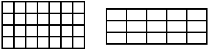
Figure 1 2D regular grids; the left one is an aa-grid (Cartesian), the right one is an ab-grid
We should mention another (equivalent) definition of the tesselations in figure 1. The Cartesian grid can be seen as a rectangle with integer edge lengths and area \(~n~\). The non-Cartesian grid can be seen as a rectangle with edge lengths \(~(m_1,~m_2 \cdot b)~\) and irrational \(~b~\), or with edge lengths \(~(m_1 \cdot a,~m_2 \cdot b)~\) and incommensurable \(~a,~b~\). In both cases is \(~m_1 \cdot m_2=n~\) with integer \(~m_1,~m_2~\). – With this definition the tesselation borders inside the outer rectangle can be omitted.
In figure 2 we see 3D regular grids. These are regular honeycombs of boxes built from \(~n~\) congruent boxes with equal orientation. The left grid in figure 2 is built from cubes and called 3D Cartesian grid or aaa-grid. The grid in the middle is called aab-grid, the building blocks having edges with two different lengths. The right grid is called abc-grid, the building blocks having edges with three different lengths.
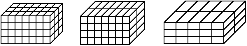
Figure 2 3D regular grids; from left to right: aaa-grid (Cartesian), aab-grid, abc-grid
An equivalent definition of the honeycombs in figure 2, similar to the 2D case, can be given. The Cartesian grid can be seen as a box with integer edge lengths and volume \(~n~\). The aab-grid can be seen as a box with edge lengths \(~(m_1,~m_2,~m_3 \cdot b)~\) and irrational \(~b~\), or with edge lengths \(~(m_1 \cdot a,~m_2 \cdot a,~m_3 \cdot b)~\) and incommensurable \(~a,~b~\). The abc-grid can be seen as a box with edge lengths \(~(m_1,~m_2 \cdot b,~m_3 \cdot c)~\) and irrational incommensurable \(~b,~c~\) or with edge lengths \(~(m_1 \cdot a,~m_2 \cdot b,~m_3 \cdot c)~\) and incommensurable \(~a,~b,~c~\). In all these cases is \(~m_1 \cdot m_2 \cdot m_3=n~\) with integer \(~m_1,~m_2,~m_3~\). – With this definition the honeycomb borders inside the outer box can be omitted.
The following sections deal with the number of ways to arrange \(~n~\) identical rectangles or boxes in regular grids, modulo rotation.
Divisors
We want to give a formula for the number of divisors of a natural number \(~n~\). This will be an essential tool for solving the problems presented at the end of the introduction. We write \(~n~\) as the unique product of its prime factors \(~p_i~\):
\[\textbf{(1)}~~~n=\prod_i p_i^{h_i}\]
The divisors of \(~n~\) can contain each prime factor \(~p_i~\) with power \(~0~...~h_i~\). So there are \(~1+h_i~\) ways for \(~p_i~\) to appear (to some power, including \(~0\)) in a divisor of \(~n~\). The number of divisors of \(~n~\) (including \(~1~\) and \(~n~\)) will be denoted by \(~\tau(n)~\) :
\[\textbf{(2)}~~~\tau(n)=\prod_i ~(1+h_i)\]
Remark: \(~n=\prod_i~ p_i^{h_i}~\) can also be read as an infinite product containing all primes \(~p_i~\) if we allow for \(~h_i=0~\). This gives a bijection between the set \(~\textbf{N}~\) of natural numbers and the sequence space \(~\textbf{N}_{\text{o}}^{\infty}~\) of all "finite" sequences of non-negative integers by the mapping \(~n \longleftrightarrow (h_i)_{i \in \textbf{N}}~\), "finite" meaning "containing finitely many non-zero members". Thus \(~\textbf{N}_{\text{o}}^{\infty}~\) is countable.
Mathematica:
\(~p_i~\) and \(~h_i~\) are given by FactorInteger[n]
\(~\tau(n)~\) is given by Length[Divisors[n]]
or f=FactorInteger[n]; le=Length[f]; Product[1+f[[m]][[2]],{m,le}]
OEIS:
\(\tau(n)~\) is given by
A000005.
2D grids (aa- and ab-grids)
The Cartesian grid in the next figure contains \(~n=28~\) squares and is a \(~(4 \times 7)-\)grid.
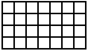
We see that \(~4 \times 7~\) can be replaced by \(~m_1 \times m_2~\) with \(~m_1,~m_2~\) divisors of \(~n~\). We want to count all ways for building these grids: As \(~m_2 = n/m_1~\) and \(~(m_1 \times m_2)-\)grids are identified with \(~(m_2 \times m_1)-\)grids, \(~m_1~\) can run through half of the divisors – but only if \(~n~\) is not a square. If \(~n~\) is a square number then a \(~(\sqrt{n} \times \sqrt{n})~-\)grid exists; this is the only case for the number of divisors being odd. We denote the number of 2D Cartesian grids with \(~n~\) squares by \(~g_{aa}(n)~\) and get:
\[\textbf{(3)}~~~g_{aa}(n)=\left\lceil \frac{\tau (n)}{2} \right\rceil\]
Remarks:
For \(~\tau(n)~\) see (2).
\(\lceil~..\rceil\) gives the smallest integer greater than or equal to the argument \(~~~\longrightarrow~~~g_{aa}(n)=(\tau(n)+1)/2~\) if \(~n~\) is a square and \(~g_{aa}(n)=\tau(n)/2~\) otherwise.
Mathematica:
\(g_{aa}(n)~\) is given by Ceiling[Length[Divisors[n]]/2]
OEIS:
\(g_{aa}(n)~\) is given by
A038548.
The non-Cartesian grid in the next figure contains \(~n=15~\) rectangles and is a \(~(3 \times 5)-\)grid.
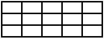
\(3 \times 5~\) can be replaced by \(~m_1 \times m_2~\) with \(~m_1,~m_2~\) divisors of \(~n~\). But in contrast to Cartesian grids \(~(m_1 \times m_2)-\)grids cannot be identified with \(~(m_2 \times m_1)-\)grids. So \(~m_1~\) can run through all divisors. We denote the number of 2D non-Cartesian grids with \(~n~\) rectangles by \(~g_{ab}(n)~\) and get:
\(\textbf{(4)}~~~g_{ab}(n)=\tau (n)~\), cf. (2)
3D Cartesian grids (aaa-grids)
The Cartesian grid in figure 3 contains \(~n=84~\) cubes and is a \(~(4 \times 7 \times 3)-\)grid.
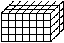
Figure 3 aaa-grid
As in the similar 2D case \(~(m_1 \times m_2 \times m_3)-\)grids are identified with \(~(m_1 \times m_3 \times m_2)-\)grids, and so on for other permutations of the three divisors. So we look for divisors satisfying \(~m_1 \leq m_2 \leq m_3~\). We denote the number of 3D Cartesian grids made from \(~n~\) cubes by \(~g_{aaa}(n)~\). We know no formula for \(~g_{aaa}(n)~\).
Mathematica:
\(g_{aaa}(n)~\) is given by
b=0; d=Divisors[n]; r=Length[d];
Do[If[d[[h]] d[[i]] d[[j]]==n, b++], {h, r}, {i, h, r}, {j, i, r}];
b
OEIS:
\(g_{aaa}(n)~\) is given by
A034836.
aab-grids
The non-Cartesian \(~(4 \times 7 \times 2)-\)grid in figure 4 is an aab-grid containing \(~n=56~\) congruent boxes with edges of two different lengths.
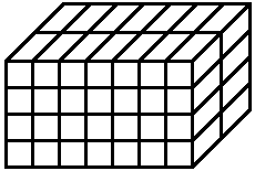
Figure 4 aab-grid
An easy way for determining the number of different aab-grids is to add up all Cartesian 2D grids – the "front" of the box in figure 4 (with squares) may serve as an example. What does "all" mean here? The 2D grid must contain \(~m~\) squares with \(~m|n~\) (\(m~\) is a divisor of \(~n\)). We denote the number of aab-grids with \(~n~\) boxes by \(~g_{aab}(n)~\). Using (3) we get:
\[\textbf{(5)}~~~g_{aab}(n)=\sum_{m|n} g_{aa}(m)=\sum_{m|n}~\left\lceil \frac{\tau (m)}{2} \right\rceil\]
Mathematica:
\(g_{aab}(n)~\) is given by
d=Divisors[n]; r=Length[d];
Sum[Ceiling[Length[Divisors[d[[j]]]]/2],{j, r}]
OEIS:
\(g_{aab}(n)~\) is given by
A140773.
abc-grids
The non-Cartesian \(~(3 \times 5 \times 2)-\)grid in figure 5 is an abc-grid containing \(~n=30~\) congruent boxes with edges of three different lengths.
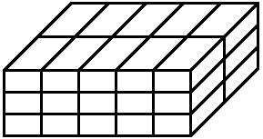
Figure 5 abc-grid
We denote the number of abc-grids with \(~n~\) boxes by \(~g_{abc}(n)~\).
We want to show that \(~g_{abc}(n)~\) equals the number of divisors of divisors of \(~n~\). This means we have to check each divisor \(~m~\) of \(~n~\) and determine the number \(~\tau (m)~\) of divisors of \(~m~\). All these numbers add up to \(~g_{abc}(n)~\).
Look at one of the faces of the box in figure 5, e.g. the "front" with \(~15~\) rectangles. The number of these rectangles must be a divisor of \(~n~\), and each divisor of \(~n~\) must be considered because the faces are non-Cartesian 2D grids; cf. the explanations leading to (4). Let \(~m~\) be such a divisor. \(~m~\) stands for the number of rectangles in a \(~(k \times m/k)-\)grid with \(~k|m~\). So for each divisor \(~m~\) of \(~n~\) we get \(~\tau (m)~\) different abc-grids. This settles our claim.
What was shown amounts to the realization that we need to look at only one face of the box — as the number \(~n/m~\) of layers "behind" it is determined by the number \(~m~\) of rectangles on the face. This number is a divisor \(~m~\) of \(~n~\), and \(~m~\) can be split into \(~k \cdot (m/k)~\) with \(~k|m~\) in order to build a rectangle for the face. We get a \(~(m_1 \times m_2 \times m_3)-\)grid with \(~(m_1 \times m_2 \times m_3)=(k \times (m/k) \times (n/m))~\) where any permutation of the \(~m_i~\) results in a different grid.
\(m|n~\) can be written as \(~m=\prod_{i=1}^s p_i^{v_i}~\) with \(~0 \leq v_i \leq h_i~\), see (1), and any such tuple \(~(v_i)_{~i=1~..~s}~\) gives a divisor \(~m~\) of \(~n~\). \(~m~\) has \(~\tau(m)=\prod_{i=1}^s~(1+v_i)~\) divisors, see (2). With this we get:
\[g_{abc}(n)=\sum_{0\leq v_i \leq h_i}~\prod_{i=1}^s ~(1+v_i)=\sum_{v_1=0}^{h_1}~\sum_{v_2=0}^{h_2}~...\sum_{v_s=0}^{h_s}~\prod_{i=1}^s ~(1+v_i)=\sum_{v_1=0}^{h_1}(1+v_1) \sum_{v_2=0}^{h_2}(1+v_2)~...\sum_{v_s=0}^{h_s}(1+v_s)\]
\[\textbf{(6)}~~~g_{abc}(n)=\prod_{i=1}^s~\binom{2+h_i}{2}\]
Mathematica:
\(g_{abc}(n)~\) is given by Length[Flatten[Divisors[Divisors[n]]]]
or f=FactorInteger[n]; r=Length[f]; Product[Binomial[2+f[[m]][[2]],2],{m, r}]
OEIS:
\(g_{abc}(n)~\) is given by
A007425.
Comments are welcome.
Last update 2022-01-18
blog overview | previous article | next article
Manfred Börgens | main page
 MB Matheblog # 17
 deutsche Version